Welcome to BandLab, the scientific software for Windows systems that performs electronic structure calculations of crystalline solids. BandLab is a library dynamically linked to MStudio. BandLab also uses MScene library for visualization.

BandLab consists of a window that is used to set up input data, perform calculations and analyze output data. The BandLab Window, shortly Bands Window is called using Bands command of the Project menu or corresponding button of the Bands Toolbar. The Bands window consists of several Property Pages:

Atoms Pagebandlab_atoms_overview
Hoppins Pagebandlab_hoppings_overview
Hubbards Pagebandlab_hubbards_overview
Properties Pagebandlab_properties_overview

A lower area of the Bands Window is an output area where the output of the calculation is shown.

The engine of the BandLab is a program called LmtART.bandlab_lmtart_overview The LmtART is an executable file that reads the input data, performs band structure calculation, and stores the output files. The Bands Window only controls this process, it prepares input for the LmtART using dialog windows, and starts LmtART program as a separate thread. When the calculation is finished, LmtART notifies the BandLab, and the output files are read by the Bands Window and can be visualized by simple mouse click operations.

While running LmtART program for complicated compounds can be rather slow (it depends how many atoms per unit cell is chosen), the BandLab can be used to prepare the input files, after which they can be copied to another computer where the LmtART can be run in a faster way. After run is performed, the output files can be copied back to the PC and BandLab can analyze them quickly. All input/output files are formatted, and therefore system independent.

The BandLab uses scratch directory to run LmtART program. By default scratch directory is called LmtRUN. It exists at the MStudio installation directory. All input/output files prepared by the Bands window are stored in this directory.

A separate issue of the BandLab is its Materials Database. The BandLab has a database of compounds that have been calculated using the LmtART program. The database is an important part of the library, it can be called by pressing DataBase button located on the top right part of the Bands Window. The input/output files can be stored within the database: this gives possibility to use these files on the remote machines. Refer to Using DataBasebandlab_database_overview topic for the detailed discussion.

2. Setting Atomic Data: Overview

Atomic data set-up is the primary set of data describing the crystalline solid. The first property page of the Bands Window is designed to describe these parameters:

Lattice parameter in atomic units
B/A and C/A ratios if the lattice has orthorhombic distortions
Primitive translations in units of lattice parameter
Spin polarization, if necessary
Spin-orbit coupling, if necessary
Temperature.

More options can be accessed via clicking Access All Options button. The corresponding property pages are

General PropertiesHIDD_ALL_OPTIONS_GENERAL
Structure PropertiesHIDD_ALL_OPTIONS_STRUCTURE
Common Tasks PropertiesHIDD_ALL_OPTIONS_TASKS

The following set of data has to be given for each atom in the unit cell

Element title, like Na, Nb, etc.
Nuclear charge. This is the most important parameter over which the software recognizes the atoms.
Position of atom in the unit cell in the units of lattice parameter.
If several atoms have the same type, specify it in the Sort column. This will be used to determine crystal group. For example, the compound YBa2Cu3O7 has 12 atoms. At the same time there only 8 nonequivalent atoms: Y, Ba, Cu1, 2*Cu2, 2*O1, 2*O2, 2*O3, and O4. Therefore, sort column will be 1 for Y@1, 2 for Ba@2, 2 for Ba@3, 3 for Cu1@4, 4 for Cu2@5, 5 for O1@6, 5 for O1@7, 6 for O2@8, 6 for O2@9, 7 for O3@10, 7 for O3@11, 8 for O4@12. Here El@N shortly denotes the element at position N.
The radius of the MT sphere can be optionally specified if this value is known. If this value is unknown, it can be computed by the LmtART.

Additional options for atoms can be accessed by highlighting the entire row and calling the Properties dialog box with the right mouse button.

Another possibility to call the Atom Properties dialog box is to access it from the Object Explorer.

The dialog box which allows to access various properties for the selected atom appears. These properties include:

General Properties
Magnetic properties
Valence States proeprties
Semicore States properties
Deep core states properties

3. Setting Hopping Integrals: Overview

Hopping integrals are necessary if tight-binding (possibly non-orthogonal) calculations of the electronic structure are desired. Tight-binding picture is an important step in understanding chemical bonding of the materials. After performing full band structure calculations, construction of simple tight-binding models describing complicated spaghetti of bands is extremely useful.

The BandLab offers two ways of working with tight-binding.

The first way is to perform band structure calculation and withdraw tight-binding integrals. This can be performed using so called tight-binding LMTO representation used by the LmtART program. A drawback of this approach is that too many hopping integrals are usually withdrawn; therefore manual analysis is required after that to select only important hoppings. Advantage of this approach is that the correct orders of magnitudes for all hoppings are obtained.
The second way is to enter hopping integrals from the terminal and try to fit the electronic structure by changing the input values Advantage of this approach is that only several hoppings integrals are varied. A drawback of it is that the significant hoppings have to be known before the analysis is performed.

Both ways require quick recalculation and drawing of the band structure using a set of hoppings, and the BandLab offers the fastest way of operating with these problems.

Usually, if building tight-binding picture for the material is necessary, one first performs the computation of all possible hopping integrals, and then manually selects the largest hoppings. The unimportant hoppings can be erased from the hoppings table and few-parameter model can be constructed.

The following inputs are required to work with the hoppings:

Cluster size: this is the size of the nearest neighbor sphere surrounding every atom. Normally only first nearest neighbors are important to consider. The hoppings between these nearest neighbors will be considered.
Filling: this is number of electrons to find the position of the Fermi level.
Tight-binding basis: set orbitals which represent tight-binding basis. For example, for CuO2 plane of YBa2Cu3O7, 3d electrons of Cu and 2p electrons of O should be considered. Syntax used for setting the orbital is El@N::nl with El is an element title, N is the position number, n is the main quantum number and l is the orbital quantum number. For example CuO2 plane is represented by Cu@1::3d orbital and O@2::2p, O@3::2p oxygen orbitals.
The use of the local coordinate system for every atom can be set in the following columns of this table. Refer to the LmtART manual for the detailed set-up of these data.
Irreducible hopping integrals have to be specified in the lower table. Term irreducible refers to those hoppings that cannot be obtained by applying group operation. In order to find irreducible hoppings automatically for given cluster and orbitals, click Irreducible button. Note that the cluster size and the orbitals have to be set up while the hopping table should be completely empty in order to perform this operation. (You should manually erase all hoppings from the table if its contents is not empty since the program does not overwrite the existing data.)
The hoppings are given FROM a particular orbital TO another orbital VIA connection vector. The value of hopping and possibly the overlap integral can be specified. Term orbital here refers to a particular lm-orbital. These, for example, will be Cu@1::3d{xy}, Cu@1::3d{yz}, Cu@1::3d{zx}, Cu@1::3d{x2-y2}, Cu@1::3d{3z2-1}, total 5 orbitals for Cu 3d basis. If the connection vector is set to 0,0,0 the hopping is reduced to the level position for this particular orbital. The overlap integral can be set to 1 in this case. For non-zero connections, the overlap integral can be set to zero if orthogonal tight-binding is considered.

It is important to understand that the tight-binding basis in this set-up considers all (2l+1) orbitals for given l-shell, not only selected components. This is done for easy transformation between cubic and spherical harmonics as well as to perform rotations to local coordinate systems. In the example of CuO2, it is well known that only Cu@1::3d{x2-y2}orbital is in fact the only important one. To take this into account shift the positions of other orbitals, Cu@1::3d{xy}’s and Cu@1::3d{3z2-1} by some amount either above or below, and do not specify hoppings from that orbitals. They will be resolved as levels and will not play any role in the tight-binding model constructed.

For spin-polarized and possibly spin-orbit coupled set-ups, the following syntax for orbitals definitions should be used: El@N-up::nl{…} or El@N-dn::nl{…}. These are, for example, Cu@1-up{x2-y2} and Cu@1-dn{x2-y2} orbitals.

Note finally that if the hopping integral is not specified within the table, its value is assumed to be equal zero.

The properties for the tight binding orbitals can be accessed via calling Properties Dialog Box. To call this dialog box select given tight-binding state and call pop-up menu by the right mouse button.

Another way to call this dialog box is to find the tight binding state at the object explorer and double click on it or call the pop-up menu using the right mouse button.

The dialog box which allows to further customize the properties of the tight-binding state will appear. It contains the following property pages

General PropertiesHIDD_SETHSTATE_GENERAL
Rotate PropertiesHIDD_SETHSTATE_ROTATE

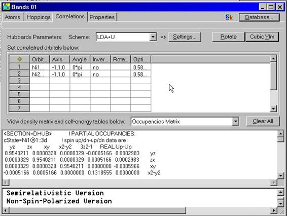
4. Setting Correlations: Overview

Correlations among d- or f-electrons in solids are important for determining their physical properties. Local density and generalized gradient approximations do not treat properly systems with the correlated electrons. A classical example of the failure is Mot-Hubbard insulator NiO. BandLab currently offers LDA+U scheme for including the effects of strong correlations into account. way of operating with these problems.

The following inputs are required to set up correlations:

Basis set for correlated orbitals: set orbitals which represent tight-binding basis. For example, for Mott-Hubbard insulator NiO, 3d electrons of Ni can be considered. Syntax used for setting the orbital is the same as for setting hopping integrals. El@N::nl with El is an element title, N is the position number, n is the main quantum number and l is the orbital quantum number. For example Ni 3d orbitals are represented by Ni@1::3d and Ni@2::3d.
The use of the local coordinate system for every atom can be set in the following columns of this table. Refer to the LmtART manual for the detailed set-up of these data.
Slater integrals should be specified in the Options column. There must be total l+1 number for given l-orbital. For d-electrons these are F0, F2, and F4 parameters.

The properties for the correlated orbitals can be accessed via calling Properties Dialog Box. To call this dialog box select given correlated state and call pop-up menu by the right mouse button.

Another way to call this dialog box is to find the tight binding state at the object explorer and double click on it or call the pop-up menu using the right mouse button.

The dialog box which allows to further customize the properties of the correlated state will appear. It contains the following property pages

General PropertiesHIDD_SETCSTATE_GENERAL
Rotate PropertiesHIDD_SETCSTATE_ROTATE
Correlations PropertiesHIDD_SETCSTATE_CORRELATIONS

When self-consistent calculation using LDA+U is done, a set of density matrices and orbital-dependent corrections to the potential are calculated. They can be analyzed in the lower part of the Correlations window.

5. Computing Physical Properties: Overview

Computation of physical properties is the goal of the BandLab library. The LmtARTbandlab_lmtart_overview program is the executable module that does this calculation. It reads input files prepared by the bands Window, performs the calculation of the desired property, and notifies the Bands Window again that the calculation is finished. The BandLab reads the output files and visualizes them with help of the MScene library.

The purpose of the Properties page of the Bands Window is to make final preparations before starting LmtART, start LmtART code, and visualize the output data computed by the LmtART. Once the compound data, and, optionally, hopping integrals are specified using Atomsbandlab_atoms_overview, Hoppingsbandlab_hoppings_overview and Correlationsbandlab_hubbards_overview property pages, the last step is to choose the method of computing the physical property.

Three methods are currently available within the use of BandLab library:

Full potential LMTO method for electronic structure calculation. This is the most precise approach for computing physical properties such as one-electron structure, but at the same time, it is computationally slow approach.
ASA-LMTO method for electronic structure calculation. This is a fast method, but less accurate comparing to the full potential LMTO method.
Tight-binding method. This method uses the hopping integrals given in the Hoppingsbandlab_hoppings_overview property page and can be used to solve few-band model Hamiltonians.

Each method has its own set of options which can be set by clicking Method Settings A more complete set of options can be accessed via clicking All Options button. It includes

Control parametersHIDD_METHOD_CTRL
Exchange correlation choiceHIDD_METHOD_EXCH
Convergence criteriaHIDD_METHOD_CONV
Mixing optionsHIDD_METHOD_MIXS
LMTO optionsHIDD_METHOD_LMTO
K-intergration settingsHIDD_METHOD_KINT
Plane wave fast fourier transform settingsHIDD_METHOD_FFTS

Both full potential LMTO and ASA LMTO methods require self-consistent calculation to be performed before computing any physical property such as the band structure or density of states. To make self-consistency, switch on radio button Make Self-Consistency and click Compute button. The self-consistent calculation will start. The output window in the lower part of the Bands Window will show haw the self-consistent process is performed. This however maybe rather slow process especially when compounds with many atoms are considered. At the end of the calculation, the framework creates the file consisting the self-consisting charge density.

Once self-consistency is performed, such physical properties as Fat Bands analysis or Density of States can be computed. One can also compute Hopping integrals necessary to build the tight-binding model.

To compute physical property such as Fat Bands, set radio button Find Property to the On position. Chose Fat Bands property from the drop-down list and press Compute button. ( You may also use Prepare button to set more options before pressing compute button.)

The following set of properties can be computed by the BandLab:

Atoms & StructureHIDD_COMPUTE_ATM
Crystal GroupHIDD_COMPUTE_GRP
Charge DensityHIDD_COMPUTE_SCF
Fat BandsHIDD_COMPUTE_FAT
Density of StatesHIDD_COMPUTE_DOS
HoppingsHIDD_COMPUTE_HOP
OpticsHIDD_COMPUTE_OPT
Full PotentialHIDD_COMPUTE_POT
Fermi SurfaceHIDD_COMPUTE_FRS

After the computation of a particular property is finished, the framework will add this into the computed properties list of the Visualize Property drop-down list.

To start visualizing the properties that have been computed, choose radio button Visualize Property. Highlight corresponding property and press Visualize button. A visualization dialog box appears. You can start visualizing the data by pressing Visualize with the current settings button in the lower part of this dialog box.

Such features as band characters can be visualized readily by the BandLab. The visualization dialog box contains a tree of atomic orbitals whose characters can be visualized within the band structure plot. To be able to visualize a particular character, drug the corresponding icon and drop it into the tree item describing the plot such as E(k) or DOS. You can choose several orbitals to be visualized at the same time. After, the band characters to be visualized are selected, press Visualize with the current settings button in the lower part of this dialog box. The Plot Page with the details of the band structure and the characters should appear.

The following controls help to visualize the computed properties:

Visualzing Atoms & StructureHIDD_VISUALIZE_ATM
Visualizing Crystal GroupHIDD_VISUALIZE_GRP
Visualizing Density of StatesHIDD_VISUALIZE_DOS
Visualizing Energy Bands and Partial CharactersHIDD_VISUALIZE_FAT
Visualizing Fermi SurfacesHIDD_VISUALIZE_FRS
Visualizing OpticsHIDD_VISUALIZE_OPT
Visualizing Full PotentialHIDD_VISUALIZE_POT
Visualizing Charge DensityHIDD_VISUALIZE_SCF

All visualization plots can be additionally customized using the commands of MScene library. Refer to the MScene Library documentation for corresponding instructions.

6. Using Materials Data Base: Overview

Materials database is important part of the BandLab library. Instead of maintaining its own input files, one can use database to extract set-ups for similar materials and then slightly modify them. After computation of the material properties and or self-consistency process is performed one can store the computed data into the database to be able to use them in the future runs.

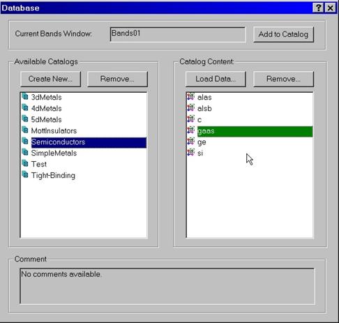
To call database press Database button located at the top right part of the bands window. The database dialog box appears. The database consists of catalogs and their contents. A set of predefined catalogs describing set-ups for 3d, 4d, 5d, simple metals, etc is provided with this installation.

To load data from the database into the Bands Window select a particular compound and press Load Data button. To store data computed by the Bands Window, use button Add to Catalog located on the top of the database dialog box.

New catalogs can be created and removed. Entries within the catalog can also be removed using corresponding buttons.

In fact, the database maintained by the framework is located in the database folder of the directory where installation of MStudio has been performed. Navigate database folder, the input and output files for many different examples are stored in its subdirectories. All these files are either input or output files of the LmtARTbandlab_lmtart_overview program that performs actual computations. Refer to the LmtART manual for detailed instructions about input and output to this program.

7. LmtART program

LmtART is free scientific software designed to perform electronic structure calculations of the materials. It is written using Fortran 90 programming language and uses full dynamical memory model. The source codes for that program, as well as installation and operating instructions can be downloaded from the same site as the MStudio, MScene and BandLab program. Refer to specific license agreement and copyright notice when using LmtART codes.

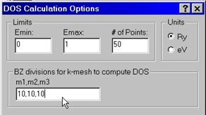
A.1 Computing Density of States

To compute density of states you need to enter minimum and maximum energies in either Ry or eV as well as # of intervals to divide the energy range Emax – Emin. You also have an option to enter # of divisions for the Brillouin zone, e.g., 10,10,10 which supersedes the input given anywhere else.

The program computes and stores the file with an extension .dos which can be further visualized.

A.2 Computing Energy Bands and Partial Characters

Energy bands can be computed along high-symmetry directions. For simple lattices like bcc,fcc, hcp, simple cubic, etc. these high symmetry directions are listed in the files str.* located in the atomdat directory. To compute energy bands and partial characters you need to enter # the number if intervals to divide every high-symmetry line. The default # is 20. If you wish to compute the energy bands in a set of custom directions, use the corresponding table control to enter Cartesian coordinates for every k-point and their notations. For example, enter in each row: g 0,0,0 ; X 0,0,1, L 0.5,0.5,0.5 to compute the energy bands along g-X-L direction. Tip: use g to denote G point. When entering the coordinates, do not take into account b/a, c/a ratios, they will be accounted for automatically.

The program computes and stores the file with an extension .fat which can be further visualized.

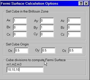
A.3 Computing Fermi Surfaces

To compute Fermi surface you need to set up a cube in the reciprocal space for which the grid of k-points will be generated and the band structure will be computed as E_j(kx,ky,kz). Then, the software will draw a cross-section E_j(kx,ky,kz)=E_f for all bands j which cross the Fermi level.

To set up the cube, enter three vectors defining the cube (e.g., 100,010,001) and the origin point (e.g. 0.5,0.5,0.5). Every k-point will be computed as the cube point minus the origin vector. Note that b/a and c/a ratios will be taken into account automatically.

You also have an option to enter # of divisions for the Brillouin zone, e.g., 10,10,10 which supersedes the input given anywhere else.

The program computes and stores the file with an extension .frs which can be further visualized.

A.4 Computing Crystal Group

To compute crystal group, there is no optional input parameters. The program stores file with the extension .grp which can be further visualized.

A.5 Computing Atoms & Structure

To compute atoms & structure, there is no optional input parameters. The program stores file with the extension .atm which can be further visualized.

A.6 Computing Hoppings Integrals

To compute atoms & structure, there is no optional input parameters. The program computes hoppings table and overwrites the table given within the bands window.

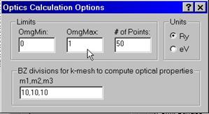
A.7 Computing Optics

To compute optical frequencies you need to enter minimum and maximum frequencies in either Ry or eV as well as # of intervals to divide the energy range Emax – Emin. You also have an option to enter # of divisions for the Brillouin zone, e.g., 10,10,10 which supersedes the input given anywhere else.

The program computes and stores the file with an extension .opt which can be further visualized.

A.8 Computing Full Potential

To compute full potential, there is no optional input parameters. The program stores file with the extension .pot which can be further visualized.

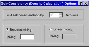
A.9 Computing Charge Density

Charge density is computed self-consistently, therefore this is the most time-consuming step in the calculation. You need to enter total # of iterations to perform the self-consistent calculation as well as mixing scheme. You have an option to select Broyden mixing which usually speeds up the self-consistent cycle significantly. If you feel this scheme does not work and you cannot get convergent result, use linear mixing scheme.

B.1 Visualizing Density of States

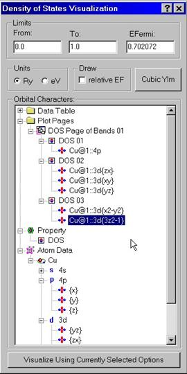
In order to visualize density of states and partial contributions, use Visualize Density of States dialog box. Enter lower and upper energy limits as well as the position of the Fermi energy in either Ry or eV. A special tree control exists to set up which partial characters should be drawn on top of the density of states. Drag partial characters from the Atomic Data folder and drop them within the Page folder into the icon showing the DOS property. Note that you can use right mouse button to access to the pop-up menu with Rename, Delete, Add commands. You can add new Pages and drag calculated properties to every of these pages. You can also put partial characters into the calculated properties by dragging them from the Atomic Data folder. In this way, you can set up spontaneously several pages with each page containing several graphs. When you are done with the descriptions of graphs, press Visualize button at the button. The program will use the graphical library to draw selected set of properties.

B.2 Visualizing Energy Bands and Partial Characters

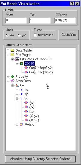In order to visualize energy bands and their partial characters, use Visualize Energy Bands dialog box. Enter lower and upper energy limits as well as the position of the Fermi energy in either Ry or eV. A special tree control exists to set up which partial characters should be drawn on top of the energy bands. They will be shown as fat lines. Drag partial characters from the Atomic Data folder and drop them within the Page folder into the icon showing the E(k) property. Note that you can use right mouse button to access to the pop-up menu with Rename, Delete, Add commands. You can add new Pages and drag calculated properties to every of these pages. You can also put partial characters into the calculated properties by dragging them from the Atomic Data folder. In this way, you can set up spontaneously several pages with each page containing several graphs. When you are done with the descriptions of graphs, press Visualize button at the button. The program will use the graphical library to draw selected set of properties.

B.3 Visualizing Fermi Surfaces

In order to visualize Fermi surface, use Visualize Fermi Surface dialog box. Enter the position of the Fermi energy in either Ry or eV. Fermi velocities can be shown either by color on top of the surface, or by vectors. When you are done with the description of graphs, press Visualize button at the button. The program will draw a multi-sheet cross-section showing the solution of the equation Ej(kx,ky,kz)=Ef.

B.4 Visualizing Crystal Group

The program shows the table containing the description of the group elements. The description for every element contains a rotation by an angle around an axis as well as whether inversion is applied after the rotation. For non-symmorphic groups a shift may also exist which is applied after the rotational operation. To see schematically the group element press the row button within the group table.

B.5 Visualizing Optics

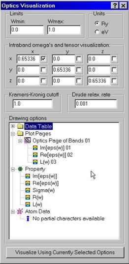In order to visualize optical properties, use Visualize Optics dialog box. Set lower and upper frequency limits for optics visualization in either Ry or eV. Since intraband contribution involves calculated plasma frequencies, you can alter them using the corresponding edit fields. Dielectric function is in general a matrix with the Cartesian components xx,xy,xz,yx,yy,yz, zx,zy,zz. Check corresponding boxes to set which of the components should be visualized. To compute real part of the dielectric function, Kramers-Kronig relationship is used. You have an option to enter upper frequency limit to use in the Kramrers-Kronig relationship. You have also an option to use a finite relaxation rate to be used in the Drude intraband contribution. When you are done with the description of graphs, press Visualize button at the button.

B.6 Visualizing Full Potential

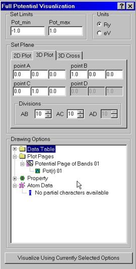Full potential can be visualized either along a set of lines, within a plane as a 2D surface or as a cross-section which is the solution of the equation V(r)=const. For spin polarized calculations you can also draw exchange-correlation magnetic fields. Without spin-orbit coupling there is only field along z-direction which is the difference between spin up and spin down potentials. If spin-orbit coupling is taken into account there are also fields along x, and y directions.

To set up a set of lines, plane or a cube, use Cartesian coordinates for the points A, B, C and D. Enter # of divisions to divide intervals AB, AC, (for the line and the plane) and AD (for the cube). Note that b/a and c/a ratios will be taken into account automatically.

The program will draw a 2D surface V(x,y). for the PLANE option. Note that we define x-axis here as left right axis, and we define y-axis here as far-near axis. The latter redefines the set of the MScene library where y-axis is defined as bottom –top axis. We use corresponding layer-mapping control to set up proper definitions. The same is true when V(x,y,z)=const. (CUBE option) is used. The program will draw the cross-section within the selected cube. The program also shows the positions of atoms by colored balls.

If magnetic field is calculated, it can be visualized as well. The magnetic field can be shown by color, symbols, or as a vector field on top of the surface. In the latter case, the maximum value of the vector length is calculated for the entire set of data. For a particular data points selected by the surface sometimes it may be too small.

If vectors did not appear, one has to rescale the lengths of the vectors to achieve a desired effect. Find the surface at the data explorer and use vectors property page to rescale their length and customize the appearance.

B.7 Visualizing Charge Density

Charge density can be visualized either along a set of lines, within a plane as a 2D surface or as a cross-section which is the solution of the equation r(r)=const. For spin polarized calculations you can also draw magnetization fields. Without spin-orbit coupling there is only magnetization along z-direction which is the difference between spin up and spin down densities. If spin-orbit coupling is taken into account there are also magnetizations along x, and y directions.

The program will draw a 2D surface r(x,y). for the PLANE option. Note that we define x-axis here as left right axis, and we define y-axis here as far-near axis. The latter redefines the set of the MScene library where y-axis is defined as bottom –top axis. We use corresponding layer-mapping control to set up proper definitions. The same is true when r(x,y,z)=const. (CUBE option) is used. The program will draw the cross-section within the selected cube. The program also shows the positions of atoms by colored balls.

If magnetization is calculated, it can be visualized as well. The magnetization can be shown by color, symbols, or as a vector field on top of the surface. In the latter case, the maximum value of the vector length is calculated for the entire set of data. For a particular data points selected by the surface sometimes it may be too small.

If vectors did not appear one has to rescale the lengths of the vectors, to achieve a desired effect. Find the surface at the data explorer and use vectors property page to rescale their length and customize the appearance.

B.8 Visualizing Atoms & Structure

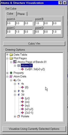Positions of atoms and various atomic orbitals can be drawn for a given crystal structure. The structure can be shown either within a cube or for a plane. Positions of atoms are shown by colored balls. Every atom of different kind is colored differently by default. The size of every ball is computed according to its atomic sphere. If the latter ones are unknown, the balls will be drawn of the same size.

Atomic orbitals can be shown at every site of the lattice. Drag various orbitals from the Atomic Data folder and drop them within the Page folder into the icon showing the Atoms property. Note that you can use right mouse button to access to the pop-up menu with Rename, Delete, Add commands. When visualizing the orbitals atomic balls will be drawn with semitransparency.

C.1 Accessing General Properties

Describe general properties such as compound title, spin dependence, and whether to switch relativistic spin orbit coupling effects (available only when spin unrestricted treatment is used).

Also temperature in K can be set which will use finite temperature Fermi Dirac functions in the calculation.

C.2 Accessing Structural Properties

Structural parameters have to be described using this property page. Lattice parameter should be given in atomic units. b/a and c/a ratios set scaling of y and z components for primitive translations. Data box can be used to select primitive translations for most common structures.

If primitive translations are given by the angles between vectors AB, BC and CA, the translations should only set the lengths for the vectors A, B, C. After the translations read, they first will be translated into cartesian coordinates and then b/a, c/a will be applied along y and z axes, respectively.

C.3 Accessing Atoms Common Tasks

Task 1. The calculation of forces on atoms can be done by the program. Since it is relatively time consuming calculation due to incomplete basis set corrections, several options can be choosen: no force calculation (default), fast force calculation with shorter output, full force calculation with long output of all partial contributions.

Task 2. If volume compression of the lattice is required, change only the parameter V/V0. Do not change lattice constants, sphere radii and any other data.

Task 3. If straining the lattice is required, specify strain matrix here. Sample strains such as volume conserved stretching are provided. if strain is applied, it is always good idea to first find minimal non-overlapping sphere radii corresponding to the largest strain. Fix the radii and then explore strained lattice for different strains with the fixed spheres.

D.1 Setting General Properties for an Atom

For each atom, several properties can be specified. The main property is atomic charge and its position in the lattice. The position can be given in Cartesian coordinates (Tx, Ty, Tz) or within the coordinate system set by the primitive translations A, B, C:

T=a*A+b*B+c*C.

Sort # should be specified such as different atoms can be of the same kind. This information will be used to find the crystal group.

Scalar relativistic effects can be utilized along with the spin orbit coupling for the valence and semicore states. The deep core states can be found using the full solution of the Dirac equation.

D.2 Setting Magnetic Properties for an Atom

To find the magnetic spin ordered solutions, the quantization axis and initial magnetic field can be given. Without spin orbit coupling effects, the quantization axis is always assumed along z direction. If spin orbit coupling is switched on, the quantization axis can align along any direction. The intial magnetic field will be switched on along magnetization axis to kick the atom out of the paramagnetic state. After that it will be switched off. This initial magnetic field is simply given by the splitting of the potential along quantization axis, for z-axis, this is simply the intial difference between spin up and spin down potentials. Note that if the atom already exists in the magnetic state, this initial splitting will be set to zero automatically unless this option is suppressed.

To apply external magnetic field along certain direction, specify the value of the field and the axis along which the external field will be switched on. The magnetic field is given in Ry and has a simple interpretation of holding spin-up and spin-down potentials to some constant value if the axis is 0,0,1

D.3 Setting Valence State Properties for an Atom

By default AtomDat directory contains the description of the valence states which will form the band structure of a given compound. If customization of these settings is required, this property page can be used.

D.4 Setting Semicore State Properties for an Atom

By default AtomDat directory contains the description of the semicore states which will form a set of narrow bands below the valence states for a given compound. If customization of these settings is required, this property page can be used.

D.5 Setting Deep Core State Properties for an Atom

By default AtomDat directory contains the description of the deep core states which will be adjusted for a given environment. If customization of these settings is required, this property page can be used.

E.1 Setting General Properties for Tight-Binding State

To calculate hopping integrals between some states, specify pointers to these states using this property page. Also specify which coordinate system to use for calculating hopping integrals, either global coordinates or local coordinates. Local coordinate system, for given atom can be set by rotating global coordinate system along a certain axis to a certain angle. Also inversion operation can be applied after such transformation.

E.2 Setting Rotate Properties for Tight-Binding State

If hopping integrals are known for some local (global) coordinate systems for each hopping state, they can also be viewed at any other coordinate system. To rotate hopping integrals for one coordinate system to another coordinate system specify the desired coordinate system using this property page. Press rotate button which should rotate the integrals within the hoppings data table to the new coordinate system and set this coordinate system as the main coordinate system.

E.3 Setting General Properties for Correlated State

To treat correlation effects for some states, specify pointers to these states using this property page. Also specify which coordinate system to use for calculating density matrices, either global coordinates or local coordinates. Local coordinate system, for given atom can be set by rotating global coordinate system along a certain axis to a certain angle. Also inversion operation can be applied after such transformation.

E.4 Setting Rotate Properties for Correlated State

If density matrices are known for some local (global) coordinate systems for each correlated state, they can also be viewed at any other coordinate system. To rotate density matrices from one coordinate system to another coordinate system specify the desired coordinate system using this property page. Press rotate button which should rotate the all matrices to the new coordinate system and set this coordinate system as the main coordinate system.

E.5 Setting Correlation Properties for Correlated State

On site correlation effects have to be described by the Slater integrals. For s state this is Hubbard constant U or Slater integral F0 which needs to be set. For p,d, f states there are additional Slater integrals which need to be set. Since correlations effects are treated on top of the LDA calculation, the double counting effects have to be taken into account. The most common choice here is U(n-1/2).

F.1 Accessing Method Controls

Various choices to adjust radial basis functions to the atomic potential can be selected here, they can either be adjusted to (spin dependent) spherical self-consistent potential, spin-averaged spherical self-consistent potential or simply found using the input spherical potential and be frozen during the self-consistent iterations.

The BandLab calculates crystal group automatically. In some cases however, one can suppress this option and use only unitary element of the group to perform the calculation. While the advantage of knowledge of the symmetry will not be utilized, this may result in suppressing numerical errors which always appear in comparing the configurations with different symmetries.

F.2 Accessing Method Exchange Correlation Functional

Different forms of both LDA and GGA exchange correlation functionals can be selected here.

F.3 Accessing Method Convergence Criteria

To limit the total number of iterations, use or interrupt the execution of self-consistent cycle when one or several criteria are achieved, specify them using this property page.

F.4 Accessing Method Mixing Options

Choose between linear and Broyden mixing schemes for calculating self-consistent charge densities. Broyden mixing is usually much faster method to find self-consistent solution but sometimes maybe unstable. Linear method is the most stable method especially when the mixing parameters are small but maybe time consuming.

F.5 Accessing LMTO Options

Use tight binding LMTO representation when calculating the hopping integrals between various states in order to build the tight-binding model for a given compound. In this case specify the cluster size within which the hopping integrals will be calculated.

Multikappa LMTO basis sets provide additional flexibility to get most accurate solutions of the problem. Usually, when using the Atomic Sphere Approximation, the number of kappa’s (LMTO tails) is set to 1 (default). For full potential LMTO method, the optimal number of kappa’s is 2 (default). Sometimes 3 can be used for most accurate calculations.

Custom tail energies (kappa’s squared) have be specified as complex numbers. For 1, 2, 3 kappa basis sets the default numbers are (-0.1,0.0), (-1.0,0.0), (2.5,0.0). If positive kappa’s are necessary, add some small imaginary part (something like 0.03) to avoid free electron singularities in the structure constants.

F.6 Accessing k Integration Options

To perform integrals over k space, select the number of divisions along reciprocal lattice vectors which will set up the grid. Different grids can be used for valence and semicore states.

The integration technique can be either tetrahedron method or Gaussian broadening method.

F.7 Accessing Plane wave FFT options

For a full potential LMTO method, the fast Fourier transform grid can be set manually. By default the program finds the FFT grid using the criterion of getting the most accurate solution. It may be too costly however for quick calculations.

Accelerations of fast Fourier transforms can be achieved for the cost of accuracy.

Accuracy in generating the pseudoHankel functions can be varied (the default value here is 0.02 for direct space and 0.04 for reciprocal space) The smaller this number, the more accurate the calculation for the cost of increasing of the amount of plane waves which will be used to expand pseudoHankel functions in Fourier series.